SNV Analysis Report
Overview
Reads Source: List of BioProject accessions
Total Samples: 9 samples
Results Directory: ../mtuberculosis/
Reference Host Genome: 2-alignment/host/genomes/Homo_sapiens_GRCh38/genome.fa
Reference Pathogen Genomes:
| Genome file | Protein file | Gene file |
|---|---|---|
| data/mycobacteriumTuberculosis/genome.fa | data/mycobacteriumTuberculosis/protein.fa | data/mycobacteriumTuberculosis/genes.gbk |
Input Reads:
| ID | Type | File 1 | File 2 |
|---|---|---|---|
| SRR25792492 | paired | data/fastq/SRR25792492_1.fastq | data/fastq/SRR25792492_2.fastq |
| SRR25792493 | paired | data/fastq/SRR25792493_1.fastq | data/fastq/SRR25792493_2.fastq |
| SRR25792494 | paired | data/fastq/SRR25792494_1.fastq | data/fastq/SRR25792494_2.fastq |
| SRR25792495 | paired | data/fastq/SRR25792495_1.fastq | data/fastq/SRR25792495_2.fastq |
| SRR25787973 | paired | data/fastq/SRR25787973_1.fastq | data/fastq/SRR25787973_2.fastq |
| SRR25787974 | paired | data/fastq/SRR25787974_1.fastq | data/fastq/SRR25787974_2.fastq |
| SRR25787975 | paired | data/fastq/SRR25787975_1.fastq | data/fastq/SRR25787975_2.fastq |
| SRR25787976 | paired | data/fastq/SRR25787976_1.fastq | data/fastq/SRR25787976_2.fastq |
| SRR25787977 | paired | data/fastq/SRR25787977_1.fastq | data/fastq/SRR25787977_2.fastq |
Read Quality
Quality Check
The quality check was done using FastQC (https://www.bioinformatics.babraham.ac.uk/projects/fastqc/). This tool analyzes the quality of all reads in fastq files and creates reports that help identify quality issues in high-throughput sequencing datasets. All the results were stored in 1-quality/fastqc.
Read Cropping
Read cropping was done using Trimmomatic (http://www.usadellab.org/cms/?page=trimmomatic). This tool preprocesses high-throughput sequencing data from next-generation sequencing platforms. It specializes in quality control and trimming of raw sequence reads, removing artifacts, adapters, and low-quality bases. When SNVGuru identifies that a read has a quality decay greater than 1.0, it crops the reads down to 100 base pairs. The cropped fastq files were stored in 1-quality/fastq.
Host Alignment
The reads were aligned against a host reference genome in order to remove reads belonging to the host instead of the pathogen, which could alter the results of the analysis. This alignment was done using STAR (https://github.com/alexdobin/STAR). This tool is a widely used RNA-seq read aligner for short and long reads, particularly well-suited for mapping reads to genomes with complex structures, such as those with many introns and alternative splicing events.. The initial alignments were stored in SAM format at 2-alignment/host/sam.
After doing this, the reads that did not align against the host reference genome were extracted using samtools (http://www.htslib.org/). First, it runs samtools view -F 256 on the SAM files, so that every sequence that aligned is ignored and the rest is saved in BAM files at 2-alignment/host/bam. Then, it runs samtools bam2fq on the resulting BAM files to transform them into fastq files. These filtered fastq files were stored at 2-alignment/host/fastq. The number of reads are the following:
| Sample | Reads Before Filter | Reads After Filter |
|---|---|---|
| SRR25787973 | 14912526 | 14782714 |
| SRR25787974 | 11072537 | 11017445 |
| SRR25787975 | 14019682 | 14006708 |
| SRR25787976 | 14982631 | 14894984 |
| SRR25787977 | 12627739 | 12573458 |
| SRR25792492 | 15396871 | 15323335 |
| SRR25792493 | 13904011 | 13637937 |
| SRR25792494 | 13689795 | 13523872 |
| SRR25792495 | 14404817 | 14397615 |
Pathogen Alignment
The reads were aligned against the provided reference pathogen genomes using HISAT2 (http://daehwankimlab.github.io/hisat2/). This tool is a widely used RNA-seq read aligner for short reads, particularly well-suited for ekaryotic transcriptomes with complex splicing patterns.. The initial alignments were stored in SAM format at 2-alignment/pathogen/sam. Then, using samtools (http://www.htslib.org/), the alignments were sorted and transformed into a BAM file running samtools sort, and finally, the MD and NM tags were added running samtools calmd. These resulting BAM files were stored at 2-alignment/pathogen/bam, where the .sorted.bam files are the result of samtools sort, and the .bam files are the final BAM files resulting from samtools calmd.
Alignment Quality
The alignments against the pathogen reference genome were analyzed using Qualimap 2 (http://qualimap.conesalab.org/). This tool inspects SAM/BAM files, analyzes the features of the mapped reads and generates a report of the aligned data. This helps detect issues in the sequencing and/or mapping of the data. The results were stored at 3-qualimap.
After the analysis is done, SNVGuru removes the samples that produced a general error rate greater than 3.0%. The error rates were the following:
| Reference pathogen | ID | Error rate (%) |
|---|---|---|
| mycobacteriumTuberculosis | SRR25792492 | 0.0 |
| mycobacteriumTuberculosis | SRR25792493 | 0.0 |
| mycobacteriumTuberculosis | SRR25792494 | 0.0 |
| mycobacteriumTuberculosis | SRR25792495 | 0.03 |
| mycobacteriumTuberculosis | SRR25787973 | 0.0 |
| mycobacteriumTuberculosis | SRR25787974 | 0.0 |
| mycobacteriumTuberculosis | SRR25787975 | 0.01 |
| mycobacteriumTuberculosis | SRR25787976 | 0.0 |
| mycobacteriumTuberculosis | SRR25787977 | 0.0 |
SNV Calling
The SNV calling step was performed using REDItools2 (https://github.com/BioinfoUNIBA/REDItools2) and JACUSA2 (https://github.com/dieterich-lab/JACUSA2).
REDItools2 is a toolkit designed for the analysis of RNA editing events in high-throughput sequencing data, identifying, quantifying, and characterizing RNA editing sites from RNA-seq data. It generates TXT files with the SNV data, which were transformed into VCF files, and these VCF files were also modified for using them as SnpEff inputs. These files were stored at 4-snvCalling/reditools. The files used for SnpEff are named as SAMPLE.reditools.presnpeff.vcf.
JACUSA2 is a framework for single nucleotide variant and reverse transcriptase induced arrest event detection in next-generation sequencing data. It generates VCF files with the SNV data, which were then preprocessed for using them as SnpEff inputs. These files were stored at 4-snvCalling/jacusa. The original output files are named as SAMPLE.jacusa.vcf. while the files used for SnpEff are named as SAMPLE.jacusa.presnpeff.vcf. There are also some files named as SAMPLE.jacusa.vcf.filtered and SAMPLE.jacusa.vcf.filtered.idx that are byproducts of the execution of the program.
Gene and Functional Effect Identification
For identifying the gene and functional effect of each SNV, the VCF files from the previous step were processed with SnpEff (http://pcingola.github.io/SnpEff/). It is a genetic variant annotation and functional effect prediction toolbox, particularly made for single nucleotide polymorphisms and small insertions/deletions. It categorizes variants based on their impact on genes, classifying them into different functional consequences such as synonymous, nonsynonymous, frameshift, and more. The output files of this tool were stored at 5-snpeff.
Allele-Specific Strand Odds Ratio Calculation
The computation of AS strand odds ratio (AS_SOR) was done executing BCFtools' (https://samtools.github.io/bcftools/) mpileup on each resulting BAM file from the alignment using the argument -a FORMAT/AD,FORMAT/ADF,FORMAT/ADR,FORMAT/DP,FORMAT/SP in order to get the allelic depth of the forward and reverse strands for both the reference and the aligned sequences. The output files are found at 4-snvCalling/depths/REFERENCE_NAME/SAMPLE_NAME.mpileup.vcf for each pathogen reference genome and sample pair.
Each output file's last column is named as the path of the respective BAM file. This column has a string that, when split by the colon (:) character, results in six fields. The fourth one is the allelic depth for the forward strand (ADF), and the fifth one is the allelic depth for the reverse strand (ARF). Both fields have two comma-separated values, where the first one corresponds to the reference allele and the second one corresponds to the alternate allele. This leaves us with four values: forward reference depth (FRD), reverse reference depth (RRD), forward alternate depth (FAD) and reverse alternate depth (RAD). The formula for calculating the AS_SOR, according to GATK (https://gatk.broadinstitute.org/hc/en-us/articles/4414586726683-AS-StrandOddsRatio) is as follows: $$AS\_SOR = {ln(\frac{FAD * RRD}{FRD * RAD}) + ln(\frac{min(FRD, RRD)}{max(FRD, RRD)}) - ln(\frac{min(FAD, RAD)}{max(FAD, RAD)})}$$ If a mutation has an AS_SOR > 4.0, then it is filtered out of the resulting files and graphs.
Results
Common Identified SNVs
This step merges the identified SNVs from JACUSA2 and REDItools2 by position and mutation (nucleotide change). If any combination of position and mutation is not found in either of the outputs, it is discarded. Furthermore, these SNVs are filtered by the following values:
- Minimum base quality: 35
- Minimum read quality: 25
- Minimum SNV coverage: 20
- Minimum main read support: 4
- Minimum SNV frequency: 0.0
These files were stored at 6-visualization/csv/globalCommon.csv for the global results among all samples, and 6-visualization/SAMPLE_NAME/csv/runCommon.csv for the results of each sample. There is also a file for the global results and for each sample of the results by JACUSA2 (6-visualization/REFERENCE_NAME/csv/globalJacusa.csv and 6-visualization/REFERENCE_NAME/SAMPLE_NAME/csv/jacusa.csv) and REDItools2 (6-visualization/csv/globalReditools.csv and 6-visualization/SAMPLE_NAME/csv/reditools.csv). Here is a sample from the global results file.
| CHROM | Position | Alt | Reference | Type | AAVar | GeneName | GeneID | RefReads | AltReads | TotalReads | Frequency | A | C | G | T | JacRefReads | JacAltReads | JacTotalReads | JacFrequency | JacA | JacC | JacG | JacT | Sample |
|---|---|---|---|---|---|---|---|---|---|---|---|---|---|---|---|---|---|---|---|---|---|---|---|---|
| AL123456.3 | 1977 | G | A | upstream_gene_variant | nan | dnaN | Rv0002 | 0 | 66 | 66 | 100.0 | 0 | 0 | 66 | 0 | 0 | 94 | 94 | 100.0 | 0 | 0 | 94 | 0 | SRR25792492 |
| AL123456.3 | 4013 | C | T | missense_variant | p.Ile245Thr | recF | Rv0003 | 0 | 138 | 138 | 100.0 | 0 | 138 | 0 | 0 | 0 | 153 | 153 | 100.0 | 0 | 153 | 0 | 0 | SRR25792492 |
| AL123456.3 | 5563 | T | G | missense_variant | p.Lys108Asn | gyrB | Rv0005 | 1132 | 4 | 1136 | 0.3520999999999999 | 0 | 0 | 1132 | 4 | 1486 | 4 | 1490 | 0.2684999999999999 | 0 | 0 | 1486 | 4 | SRR25792492 |
| AL123456.3 | 5617 | T | G | synonymous_variant | p.Ser126Ser | gyrB | Rv0005 | 1205 | 7 | 1212 | 0.5776 | 0 | 0 | 1205 | 7 | 1436 | 7 | 1443 | 0.4851 | 0 | 0 | 1436 | 7 | SRR25792492 |
| AL123456.3 | 6134 | T | G | stop_gained | p.Glu299* | gyrB | Rv0005 | 1158 | 6 | 1164 | 0.5155 | 0 | 0 | 1158 | 6 | 1344 | 6 | 1350 | 0.4444 | 0 | 0 | 1344 | 6 | SRR25792492 |
| AL123456.3 | 6178 | T | C | synonymous_variant | p.Gly313Gly | gyrB | Rv0005 | 1229 | 4 | 1233 | 0.3243999999999999 | 0 | 1229 | 0 | 4 | 1479 | 5 | 1484 | 0.3369 | 0 | 1479 | 0 | 5 | SRR25792492 |
| AL123456.3 | 6220 | T | G | synonymous_variant | p.Val327Val | gyrB | Rv0005 | 971 | 4 | 975 | 0.4103 | 0 | 0 | 971 | 4 | 1185 | 4 | 1189 | 0.3364 | 0 | 0 | 1185 | 4 | SRR25792492 |
| AL123456.3 | 6349 | T | G | missense_variant | p.Gln370His | gyrB | Rv0005 | 1468 | 4 | 1472 | 0.2717 | 0 | 0 | 1468 | 4 | 1743 | 4 | 1747 | 0.2289999999999999 | 0 | 0 | 1743 | 4 | SRR25792492 |
| AL123456.3 | 6558 | C | G | missense_variant | p.Gly440Ala | gyrB | Rv0005 | 956 | 4 | 960 | 0.4166999999999999 | 0 | 4 | 956 | 0 | 1092 | 4 | 1097 | 0.365 | 0 | 4 | 1092 | 1 | SRR25792492 |
| AL123456.3 | 6626 | C | G | missense_variant | p.Ala463Pro | gyrB | Rv0005 | 806 | 4 | 810 | 0.4937999999999999 | 0 | 4 | 806 | 0 | 1016 | 4 | 1023 | 0.3922 | 3 | 4 | 1016 | 0 | SRR25792492 |
| AL123456.3 | 7362 | C | G | missense_variant | p.Glu21Gln | gyrA | Rv0006 | 0 | 778 | 778 | 100.0 | 0 | 778 | 0 | 0 | 0 | 876 | 876 | 100.0 | 0 | 876 | 0 | 0 | SRR25792492 |
| AL123456.3 | 7585 | C | G | missense_variant | p.Ser95Thr | gyrA | Rv0006 | 0 | 525 | 525 | 100.0 | 0 | 525 | 0 | 0 | 0 | 636 | 636 | 100.0 | 0 | 636 | 0 | 0 | SRR25792492 |
| AL123456.3 | 8559 | T | G | stop_gained | p.Gly420* | gyrA | Rv0006 | 783 | 4 | 787 | 0.5083 | 0 | 0 | 783 | 4 | 912 | 4 | 916 | 0.4367 | 0 | 0 | 912 | 4 | SRR25792492 |
| AL123456.3 | 8936 | T | G | missense_variant | p.Gln545His | gyrA | Rv0006 | 901 | 4 | 905 | 0.442 | 0 | 0 | 901 | 4 | 1139 | 4 | 1143 | 0.35 | 0 | 0 | 1139 | 4 | SRR25792492 |
| AL123456.3 | 9089 | T | G | synonymous_variant | p.Val596Val | gyrA | Rv0006 | 843 | 4 | 847 | 0.4723 | 0 | 0 | 843 | 4 | 994 | 5 | 999 | 0.5005 | 0 | 0 | 994 | 5 | SRR25792492 |
| AL123456.3 | 9304 | A | G | missense_variant | p.Gly668Asp | gyrA | Rv0006 | 0 | 681 | 681 | 100.0 | 681 | 0 | 0 | 0 | 0 | 803 | 803 | 100.0 | 803 | 0 | 0 | 0 | SRR25792492 |
| AL123456.3 | 9628 | T | C | missense_variant | p.Ala776Val | gyrA | Rv0006 | 763 | 4 | 767 | 0.5215 | 0 | 763 | 0 | 4 | 1168 | 4 | 1172 | 0.3413 | 0 | 1168 | 0 | 4 | SRR25792492 |
| AL123456.3 | 9921 | T | C | missense_variant | p.Ala3Val | Rv0007 | Rv0007 | 811 | 4 | 815 | 0.4908 | 0 | 811 | 0 | 4 | 1007 | 4 | 1011 | 0.3956 | 0 | 1007 | 0 | 4 | SRR25792492 |
| AL123456.3 | 11820 | G | C | upstream_gene_variant | nan | ppiA | Rv0009 | 0 | 26 | 26 | 100.0 | 0 | 0 | 26 | 0 | 0 | 32 | 32 | 100.0 | 0 | 0 | 32 | 0 | SRR25792492 |
| AL123456.3 | 11879 | G | A | missense_variant | p.Ser145Pro | Rv0008c | Rv0008c | 0 | 30 | 30 | 100.0 | 0 | 0 | 30 | 0 | 0 | 34 | 34 | 100.0 | 0 | 0 | 34 | 0 | SRR25792492 |
| AL123456.3 | 14785 | C | T | missense_variant | p.Cys233Arg | Rv0012 | Rv0012 | 0 | 146 | 147 | 100.0 | 1 | 146 | 0 | 0 | 0 | 180 | 181 | 100.0 | 1 | 180 | 0 | 0 | SRR25792492 |
| AL123456.3 | 14785 | C | T | missense_variant | p.Cys233Ser | Rv0012 | Rv0012 | 0 | 146 | 147 | 100.0 | 1 | 146 | 0 | 0 | 0 | 180 | 181 | 100.0 | 1 | 180 | 0 | 0 | SRR25792492 |
| AL123456.3 | 14861 | T | G | missense_variant | p.Gly258Val | Rv0012 | Rv0012 | 0 | 194 | 194 | 100.0 | 0 | 0 | 0 | 194 | 1 | 224 | 225 | 99.5556 | 0 | 0 | 1 | 224 | SRR25792492 |
| AL123456.3 | 15117 | G | C | missense_variant | p.Ile68Met | trpG | Rv0013 | 0 | 258 | 258 | 100.0 | 0 | 0 | 258 | 0 | 0 | 302 | 302 | 100.0 | 0 | 0 | 302 | 0 | SRR25792492 |
| AL123456.3 | 16119 | A | C | missense_variant | p.Arg451Leu | pknB | Rv0014c | 0 | 216 | 216 | 100.0 | 216 | 0 | 0 | 0 | 0 | 246 | 246 | 100.0 | 246 | 0 | 0 | 0 | SRR25792492 |
| AL123456.3 | 18394 | A | C | missense_variant | p.Glu123Asp | pknA | Rv0015c | 697 | 4 | 701 | 0.5706 | 4 | 697 | 0 | 0 | 821 | 4 | 826 | 0.4848 | 4 | 821 | 0 | 1 | SRR25792492 |
| AL123456.3 | 19514 | A | C | stop_gained | p.Glu241* | pbpA | Rv0016c | 253 | 4 | 257 | 1.5564 | 4 | 253 | 0 | 0 | 333 | 4 | 337 | 1.1868999999999998 | 4 | 333 | 0 | 0 | SRR25792492 |
| AL123456.3 | 21795 | A | G | missense_variant | p.Pro463Ser | pstP | Rv0018c | 0 | 225 | 225 | 100.0 | 225 | 0 | 0 | 0 | 0 | 259 | 259 | 100.0 | 259 | 0 | 0 | 0 | SRR25792492 |
| AL123456.3 | 21906 | A | C | missense_variant | p.Ala426Ser | pstP | Rv0018c | 376 | 4 | 380 | 1.0526 | 4 | 376 | 0 | 0 | 461 | 4 | 465 | 0.8602000000000001 | 4 | 461 | 0 | 0 | SRR25792492 |
| AL123456.3 | 22613 | A | G | missense_variant | p.Ser190Leu | pstP | Rv0018c | 365 | 4 | 369 | 1.084 | 4 | 0 | 365 | 0 | 464 | 4 | 468 | 0.8547000000000001 | 4 | 0 | 464 | 0 | SRR25792492 |
| AL123456.3 | 23750 | A | C | upstream_gene_variant | nan | pknA | Rv0015c | 441 | 4 | 445 | 0.8989 | 4 | 441 | 0 | 0 | 590 | 4 | 594 | 0.6734 | 4 | 590 | 0 | 0 | SRR25792492 |
| AL123456.3 | 24159 | C | T | missense_variant | p.Tyr429Cys | fhaA | Rv0020c | 799 | 4 | 803 | 0.4981 | 0 | 4 | 0 | 799 | 971 | 4 | 975 | 0.4103 | 0 | 4 | 0 | 971 | SRR25792492 |
| AL123456.3 | 24532 | T | C | missense_variant | p.Gly305Ser | fhaA | Rv0020c | 0 | 804 | 804 | 100.0 | 0 | 0 | 0 | 804 | 0 | 893 | 893 | 100.0 | 0 | 0 | 0 | 893 | SRR25792492 |
| AL123456.3 | 24716 | G | A | synonymous_variant | p.Gly243Gly | fhaA | Rv0020c | 58 | 81 | 139 | 58.2734 | 58 | 0 | 81 | 0 | 101 | 249 | 350 | 71.1429 | 101 | 0 | 249 | 0 | SRR25792492 |
| AL123456.3 | 24721 | C | G | missense_variant | p.Arg242Gly | fhaA | Rv0020c | 249 | 5 | 254 | 1.9685 | 0 | 5 | 249 | 0 | 443 | 9 | 453 | 1.9912 | 1 | 9 | 443 | 0 | SRR25792492 |
| AL123456.3 | 24885 | A | C | missense_variant | p.Arg187Leu | fhaA | Rv0020c | 1101 | 4 | 1105 | 0.362 | 4 | 1101 | 0 | 0 | 1455 | 4 | 1459 | 0.2742 | 4 | 1455 | 0 | 0 | SRR25792492 |
| AL123456.3 | 25210 | A | C | stop_gained | p.Glu79* | fhaA | Rv0020c | 1116 | 4 | 1120 | 0.3571 | 4 | 1116 | 0 | 0 | 1311 | 5 | 1316 | 0.3798999999999999 | 5 | 1311 | 0 | 0 | SRR25792492 |
| AL123456.3 | 25298 | A | C | missense_variant | p.Gln49His | fhaA | Rv0020c | 947 | 5 | 952 | 0.5252 | 5 | 947 | 0 | 0 | 1196 | 5 | 1201 | 0.4163 | 5 | 1196 | 0 | 0 | SRR25792492 |
| AL123456.3 | 25447 | G | T | upstream_gene_variant | nan | rodA | Rv0017c | 0 | 246 | 246 | 100.0 | 0 | 0 | 246 | 0 | 0 | 292 | 292 | 100.0 | 0 | 0 | 292 | 0 | SRR25792492 |
| AL123456.3 | 25610 | C | G | upstream_gene_variant | nan | rodA | Rv0017c | 0 | 54 | 54 | 100.0 | 0 | 54 | 0 | 0 | 0 | 57 | 57 | 100.0 | 0 | 57 | 0 | 0 | SRR25792492 |
| AL123456.3 | 34044 | C | T | upstream_gene_variant | nan | bioF2 | Rv0032 | 0 | 23 | 23 | 100.0 | 0 | 23 | 0 | 0 | 0 | 29 | 29 | 100.0 | 0 | 29 | 0 | 0 | SRR25792492 |
| AL123456.3 | 41378 | T | G | missense_variant | p.Leu25Phe | Rv0038 | Rv0038 | 302 | 4 | 306 | 1.3072 | 0 | 0 | 302 | 4 | 344 | 4 | 348 | 1.1494 | 0 | 0 | 344 | 4 | SRR25792492 |
| AL123456.3 | 41516 | T | G | missense_variant | p.Trp71Cys | Rv0038 | Rv0038 | 430 | 4 | 434 | 0.9217 | 0 | 0 | 430 | 4 | 530 | 4 | 534 | 0.7491 | 0 | 0 | 530 | 4 | SRR25792492 |
| AL123456.3 | 42281 | A | C | missense_variant | p.Cys24Phe | Rv0039c | Rv0039c | 0 | 126 | 126 | 100.0 | 126 | 0 | 0 | 0 | 0 | 147 | 147 | 100.0 | 147 | 0 | 0 | 0 | SRR25792492 |
| AL123456.3 | 42967 | C | G | synonymous_variant | p.Pro133Pro | mtc28 | Rv0040c | 0 | 332 | 332 | 100.0 | 0 | 332 | 0 | 0 | 0 | 367 | 367 | 100.0 | 0 | 367 | 0 | 0 | SRR25792492 |
| AL123456.3 | 43732 | A | G | synonymous_variant | p.Ser57Ser | leuS | Rv0041 | 0 | 121 | 121 | 100.0 | 121 | 0 | 0 | 0 | 0 | 141 | 141 | 100.0 | 141 | 0 | 0 | 0 | SRR25792492 |
| AL123456.3 | 44768 | G | A | missense_variant | p.Arg403Gly | leuS | Rv0041 | 0 | 51 | 51 | 100.0 | 0 | 0 | 51 | 0 | 0 | 56 | 56 | 100.0 | 0 | 0 | 56 | 0 | SRR25792492 |
| AL123456.3 | 49360 | T | C | missense_variant | p.Val194Ile | Rv0045c | Rv0045c | 0 | 94 | 94 | 100.0 | 0 | 0 | 0 | 94 | 0 | 115 | 115 | 100.0 | 0 | 0 | 0 | 115 | SRR25792492 |
| AL123456.3 | 49966 | A | C | upstream_gene_variant | nan | Rv0042c | Rv0042c | 1480 | 7 | 1487 | 0.4707 | 7 | 1480 | 0 | 0 | 1648 | 7 | 1655 | 0.423 | 7 | 1648 | 0 | 0 | SRR25792492 |
| AL123456.3 | 50114 | A | C | synonymous_variant | p.Val337Val | ino1 | Rv0046c | 1609 | 4 | 1613 | 0.248 | 4 | 1609 | 0 | 0 | 1832 | 4 | 1836 | 0.2178999999999999 | 4 | 1832 | 0 | 0 | SRR25792492 |
| AL123456.3 | 50270 | A | C | missense_variant | p.Trp285Cys | ino1 | Rv0046c | 1814 | 5 | 1820 | 0.2749 | 5 | 1814 | 1 | 0 | 2310 | 5 | 2316 | 0.216 | 5 | 2310 | 1 | 0 | SRR25792492 |
| AL123456.3 | 50311 | A | C | missense_variant | p.Gly272Cys | ino1 | Rv0046c | 1769 | 4 | 1773 | 0.2256 | 4 | 1769 | 0 | 0 | 2176 | 5 | 2181 | 0.2293 | 5 | 2176 | 0 | 0 | SRR25792492 |
| AL123456.3 | 50557 | C | T | missense_variant | p.Arg190Gly | ino1 | Rv0046c | 0 | 1645 | 1645 | 100.0 | 0 | 1645 | 0 | 0 | 0 | 1753 | 1753 | 100.0 | 0 | 1753 | 0 | 0 | SRR25792492 |
| AL123456.3 | 51026 | A | G | synonymous_variant | p.Gly33Gly | ino1 | Rv0046c | 1588 | 4 | 1592 | 0.2513 | 4 | 0 | 1588 | 0 | 1796 | 4 | 1800 | 0.2222 | 4 | 0 | 1796 | 0 | SRR25792492 |
| AL123456.3 | 51142 | A | C | upstream_gene_variant | nan | Rv0042c | Rv0042c | 1018 | 5 | 1024 | 0.4888 | 5 | 1018 | 0 | 1 | 1221 | 6 | 1229 | 0.489 | 6 | 1221 | 0 | 2 | SRR25792492 |
| AL123456.3 | 51171 | A | G | upstream_gene_variant | nan | Rv0042c | Rv0042c | 712 | 5 | 717 | 0.6974 | 5 | 0 | 712 | 0 | 1018 | 5 | 1023 | 0.4888 | 5 | 0 | 1018 | 0 | SRR25792492 |
| AL123456.3 | 51551 | A | C | synonymous_variant | p.Ala59Ala | Rv0047c | Rv0047c | 1873 | 9 | 1883 | 0.4781999999999999 | 9 | 1873 | 0 | 1 | 2051 | 10 | 2062 | 0.4852 | 10 | 2051 | 0 | 1 | SRR25792492 |
| AL123456.3 | 51580 | A | C | missense_variant | p.Gly50Trp | Rv0047c | Rv0047c | 2082 | 5 | 2087 | 0.2396 | 5 | 2082 | 0 | 0 | 2265 | 5 | 2270 | 0.2203 | 5 | 2265 | 0 | 0 | SRR25792492 |
| AL123456.3 | 51694 | A | C | missense_variant | p.Glu12Lys | Rv0047c | Rv0047c | 1384 | 5 | 1390 | 0.36 | 5 | 1384 | 0 | 1 | 1686 | 5 | 1692 | 0.2957 | 5 | 1686 | 0 | 1 | SRR25792492 |
| AL123456.3 | 51694 | A | C | stop_gained | p.Glu12* | Rv0047c | Rv0047c | 1384 | 5 | 1390 | 0.36 | 5 | 1384 | 0 | 1 | 1686 | 5 | 1692 | 0.2957 | 5 | 1686 | 0 | 1 | SRR25792492 |
| AL123456.3 | 51949 | G | A | missense_variant | p.Val250Ala | Rv0048c | Rv0048c | 0 | 50 | 50 | 100.0 | 0 | 0 | 50 | 0 | 0 | 58 | 58 | 100.0 | 0 | 0 | 58 | 0 | SRR25792492 |
| AL123456.3 | 54394 | G | A | synonymous_variant | p.Ala244Ala | ponA1 | Rv0050 | 0 | 800 | 800 | 100.0 | 0 | 0 | 800 | 0 | 0 | 848 | 848 | 100.0 | 0 | 0 | 848 | 0 | SRR25792492 |
| AL123456.3 | 55553 | T | C | missense_variant | p.Pro631Ser | ponA1 | Rv0050 | 0 | 49 | 49 | 100.0 | 0 | 0 | 0 | 49 | 13 | 100 | 113 | 88.4956 | 0 | 13 | 0 | 100 | SRR25792492 |
| AL123456.3 | 59563 | T | G | missense_variant | p.Arg52Leu | rplI | Rv0056 | 351 | 5 | 356 | 1.4045 | 0 | 0 | 351 | 5 | 418 | 5 | 423 | 1.1820000000000002 | 0 | 0 | 418 | 5 | SRR25792492 |
| AL123456.3 | 59807 | T | G | synonymous_variant | p.Ser133Ser | rplI | Rv0056 | 287 | 4 | 291 | 1.3746 | 0 | 0 | 287 | 4 | 337 | 4 | 341 | 1.173 | 0 | 0 | 337 | 4 | SRR25792492 |
| AL123456.3 | 62049 | G | A | missense_variant | p.Arg552Trp | dnaB | Rv0058 | 0 | 247 | 249 | 100.0 | 0 | 0 | 247 | 2 | 0 | 300 | 302 | 100.0 | 0 | 0 | 300 | 2 | SRR25792492 |
| AL123456.3 | 62049 | G | A | missense_variant | p.Arg552Gly | dnaB | Rv0058 | 0 | 247 | 249 | 100.0 | 0 | 0 | 247 | 2 | 0 | 300 | 302 | 100.0 | 0 | 0 | 300 | 2 | SRR25792492 |
| AL123456.3 | 63146 | T | G | upstream_gene_variant | nan | Rv0059 | Rv0059 | 0 | 239 | 239 | 100.0 | 0 | 0 | 0 | 239 | 0 | 255 | 255 | 100.0 | 0 | 0 | 0 | 255 | SRR25792492 |
| AL123456.3 | 65150 | T | C | missense_variant | p.Trp67Cys | Rv0061c | Rv0061c | 0 | 471 | 472 | 100.0 | 0 | 0 | 1 | 471 | 0 | 561 | 562 | 100.0 | 0 | 0 | 1 | 561 | SRR25792492 |
| AL123456.3 | 65150 | T | C | stop_gained | p.Trp67* | Rv0061c | Rv0061c | 0 | 471 | 472 | 100.0 | 0 | 0 | 1 | 471 | 0 | 561 | 562 | 100.0 | 0 | 0 | 1 | 561 | SRR25792492 |
| AL123456.3 | 65246 | T | C | synonymous_variant | p.Gln35Gln | Rv0061c | Rv0061c | 0 | 373 | 373 | 100.0 | 0 | 0 | 0 | 373 | 1 | 477 | 478 | 99.7908 | 0 | 1 | 0 | 477 | SRR25792492 |
| AL123456.3 | 68336 | A | G | missense_variant | p.Val472Ile | Rv0063 | Rv0063 | 0 | 51 | 51 | 100.0 | 51 | 0 | 0 | 0 | 0 | 51 | 51 | 100.0 | 51 | 0 | 0 | 0 | SRR25792492 |
| AL123456.3 | 69989 | A | G | missense_variant | p.Gly457Asp | Rv0064 | Rv0064 | 0 | 470 | 470 | 100.0 | 470 | 0 | 0 | 0 | 0 | 509 | 509 | 100.0 | 509 | 0 | 0 | 0 | SRR25792492 |
| AL123456.3 | 70267 | T | G | missense_variant | p.Val550Phe | Rv0064 | Rv0064 | 0 | 423 | 423 | 100.0 | 0 | 0 | 0 | 423 | 0 | 546 | 546 | 100.0 | 0 | 0 | 0 | 546 | SRR25792492 |
| AL123456.3 | 70816 | G | A | missense_variant | p.Asn733Asp | Rv0064 | Rv0064 | 0 | 433 | 433 | 100.0 | 0 | 0 | 433 | 0 | 0 | 480 | 480 | 100.0 | 0 | 0 | 480 | 0 | SRR25792492 |
| AL123456.3 | 71336 | C | G | missense_variant | p.Arg906Pro | Rv0064 | Rv0064 | 0 | 262 | 262 | 100.0 | 0 | 262 | 0 | 0 | 0 | 289 | 289 | 100.0 | 0 | 289 | 0 | 0 | SRR25792492 |
| AL123456.3 | 71874 | T | G | missense_variant | p.Lys18Asn | vapC1 | Rv0065 | 1499 | 4 | 1503 | 0.2661 | 0 | 0 | 1499 | 4 | 1796 | 4 | 1801 | 0.2222 | 1 | 0 | 1796 | 4 | SRR25792492 |
| AL123456.3 | 71914 | C | T | missense_variant | p.Ser32Pro | vapC1 | Rv0065 | 2 | 1829 | 1831 | 99.8908 | 0 | 1829 | 0 | 2 | 2 | 2082 | 2084 | 99.904 | 0 | 2082 | 0 | 2 | SRR25792492 |
| AL123456.3 | 72003 | T | G | missense_variant | p.Gln61His | vapC1 | Rv0065 | 2274 | 8 | 2282 | 0.3506 | 0 | 0 | 2274 | 8 | 2779 | 8 | 2787 | 0.287 | 0 | 0 | 2779 | 8 | SRR25792492 |
| AL123456.3 | 72055 | T | C | missense_variant | p.His79Tyr | vapC1 | Rv0065 | 2210 | 4 | 2214 | 0.1807 | 0 | 2210 | 0 | 4 | 2665 | 4 | 2669 | 0.1498999999999999 | 0 | 2665 | 0 | 4 | SRR25792492 |
| AL123456.3 | 75940 | C | G | missense_variant | p.Val214Leu | Rv0068 | Rv0068 | 0 | 57 | 57 | 100.0 | 0 | 57 | 0 | 0 | 0 | 65 | 65 | 100.0 | 0 | 65 | 0 | 0 | SRR25792492 |
| AL123456.3 | 78636 | A | G | synonymous_variant | p.Gly87Gly | glyA2 | Rv0070c | 0 | 46 | 46 | 100.0 | 46 | 0 | 0 | 0 | 0 | 50 | 50 | 100.0 | 50 | 0 | 0 | 0 | SRR25792492 |
| AL123456.3 | 87468 | T | C | missense_variant | p.Glu112Lys | Rv0078A | Rv0078A | 0 | 254 | 254 | 100.0 | 0 | 0 | 0 | 254 | 0 | 310 | 310 | 100.0 | 0 | 0 | 0 | 310 | SRR25792492 |
| AL123456.3 | 87652 | A | G | synonymous_variant | p.Asn50Asn | Rv0078A | Rv0078A | 618 | 4 | 622 | 0.6431 | 4 | 0 | 618 | 0 | 774 | 4 | 778 | 0.5141 | 4 | 0 | 774 | 0 | SRR25792492 |
| AL123456.3 | 88269 | T | G | synonymous_variant | p.Pro22Pro | Rv0079 | Rv0079 | 4041 | 4 | 4046 | 0.0989 | 1 | 0 | 4041 | 4 | 4839 | 4 | 4844 | 0.0826 | 1 | 0 | 4839 | 4 | SRR25792492 |
| AL123456.3 | 88287 | T | C | synonymous_variant | p.Ser28Ser | Rv0079 | Rv0079 | 4337 | 4 | 4341 | 0.0921 | 0 | 4337 | 0 | 4 | 5084 | 4 | 5088 | 0.0786 | 0 | 5084 | 0 | 4 | SRR25792492 |
| AL123456.3 | 88288 | T | G | missense_variant | p.Gly29Cys | Rv0079 | Rv0079 | 4138 | 4 | 4142 | 0.0965999999999999 | 0 | 0 | 4138 | 4 | 4630 | 4 | 4634 | 0.0863 | 0 | 0 | 4630 | 4 | SRR25792492 |
| AL123456.3 | 88290 | T | C | synonymous_variant | p.Gly29Gly | Rv0079 | Rv0079 | 4254 | 7 | 4261 | 0.1643 | 0 | 4254 | 0 | 7 | 4678 | 8 | 4686 | 0.1707 | 0 | 4678 | 0 | 8 | SRR25792492 |
| AL123456.3 | 88291 | T | G | missense_variant | p.Gly30Cys | Rv0079 | Rv0079 | 4100 | 7 | 4107 | 0.1704 | 0 | 0 | 4100 | 7 | 4470 | 7 | 4477 | 0.1564 | 0 | 0 | 4470 | 7 | SRR25792492 |
| AL123456.3 | 88314 | T | C | synonymous_variant | p.Ala37Ala | Rv0079 | Rv0079 | 3836 | 4 | 3840 | 0.1042 | 0 | 3836 | 0 | 4 | 5648 | 5 | 5653 | 0.0884 | 0 | 5648 | 0 | 5 | SRR25792492 |
| AL123456.3 | 88327 | T | C | missense_variant | p.Arg42Cys | Rv0079 | Rv0079 | 4299 | 4 | 4303 | 0.093 | 0 | 4299 | 0 | 4 | 5977 | 5 | 5983 | 0.0836 | 0 | 5977 | 1 | 5 | SRR25792492 |
| AL123456.3 | 88328 | T | G | missense_variant | p.Arg42Leu | Rv0079 | Rv0079 | 4177 | 6 | 4184 | 0.1434 | 0 | 1 | 4177 | 6 | 5746 | 7 | 5755 | 0.1217 | 0 | 2 | 5746 | 7 | SRR25792492 |
| AL123456.3 | 88328 | T | G | missense_variant | p.Arg42Pro | Rv0079 | Rv0079 | 4177 | 6 | 4184 | 0.1434 | 0 | 1 | 4177 | 6 | 5746 | 7 | 5755 | 0.1217 | 0 | 2 | 5746 | 7 | SRR25792492 |
| AL123456.3 | 88333 | T | G | missense_variant | p.Val44Leu | Rv0079 | Rv0079 | 4879 | 14 | 4894 | 0.2860999999999999 | 1 | 0 | 4879 | 14 | 5856 | 18 | 5875 | 0.3064 | 1 | 0 | 5856 | 18 | SRR25792492 |
| AL123456.3 | 88333 | T | G | missense_variant | p.Val44Met | Rv0079 | Rv0079 | 4879 | 14 | 4894 | 0.2860999999999999 | 1 | 0 | 4879 | 14 | 5856 | 18 | 5875 | 0.3064 | 1 | 0 | 5856 | 18 | SRR25792492 |
| AL123456.3 | 88335 | T | G | synonymous_variant | p.Val44Val | Rv0079 | Rv0079 | 4730 | 18 | 4749 | 0.3791 | 0 | 1 | 4730 | 18 | 5355 | 19 | 5376 | 0.3536 | 0 | 2 | 5355 | 19 | SRR25792492 |
| AL123456.3 | 88336 | T | G | missense_variant | p.Gly45Cys | Rv0079 | Rv0079 | 4837 | 5 | 4842 | 0.1033 | 0 | 0 | 4837 | 5 | 5432 | 6 | 5438 | 0.1103 | 0 | 0 | 5432 | 6 | SRR25792492 |
| AL123456.3 | 88339 | T | C | missense_variant | p.Arg46Cys | Rv0079 | Rv0079 | 4806 | 4 | 4810 | 0.0832 | 0 | 4806 | 0 | 4 | 5507 | 4 | 5511 | 0.0726 | 0 | 5507 | 0 | 4 | SRR25792492 |
| AL123456.3 | 88340 | T | G | missense_variant | p.Arg46Leu | Rv0079 | Rv0079 | 4895 | 4 | 4899 | 0.0816 | 0 | 0 | 4895 | 4 | 5480 | 5 | 5486 | 0.0912 | 1 | 0 | 5480 | 5 | SRR25792492 |
| AL123456.3 | 88344 | T | G | synonymous_variant | p.Val47Val | Rv0079 | Rv0079 | 4716 | 4 | 4720 | 0.0847 | 0 | 0 | 4716 | 4 | 5455 | 4 | 5459 | 0.0733 | 0 | 0 | 5455 | 4 | SRR25792492 |
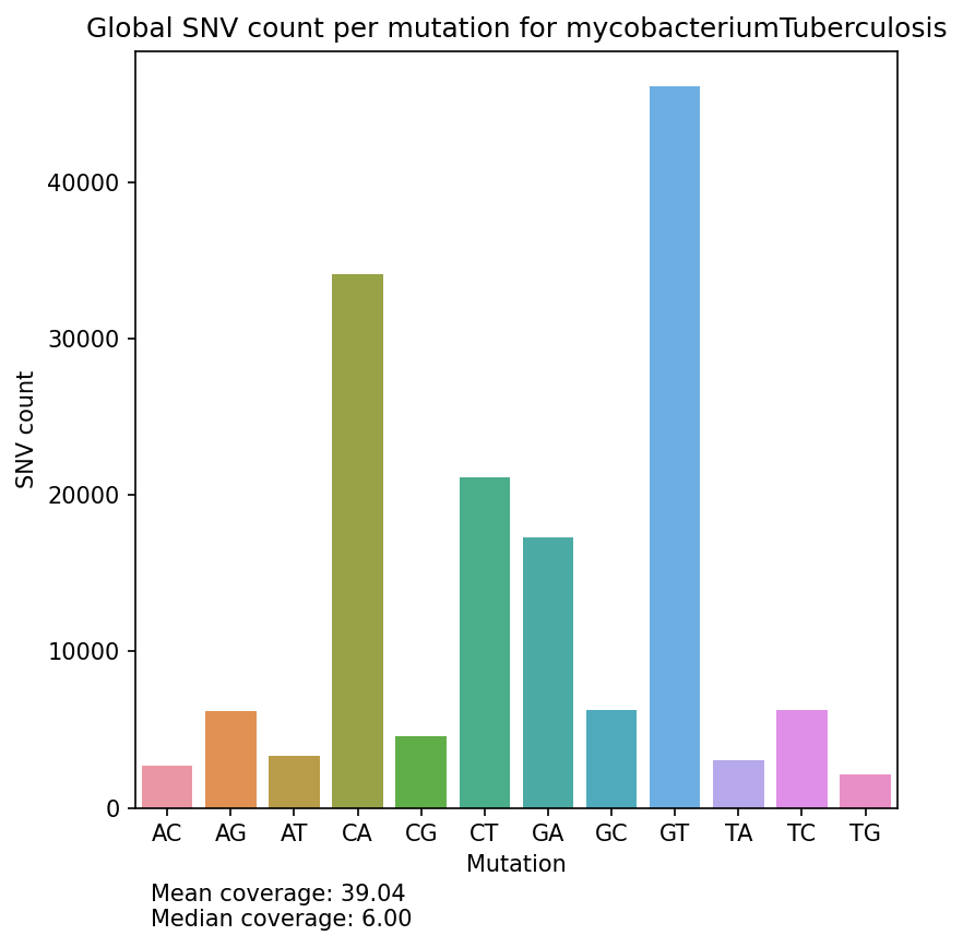
Mutation Count Bar Plot
Each sample has its own mutation count bar plot, as well as each reference pathogen genome has its own global mutation count bar plot. For each possible mutation, it counts how many times the mutation happened among all reads, regardless of the position, and plots it as a bar. It also displays the mean coverage and median coverage, where the coverage is the number of reads with alternate allele. These graphs were stored at 6-visualization/REFERENCE_NAME/graphs/common.mutationCountBarPlot.png for each reference genome graph, or 6-visualization/REFERENCE_NAME/SAMPLE_NAME/graphs/common.mutationCountBarPlot.png for each sample.
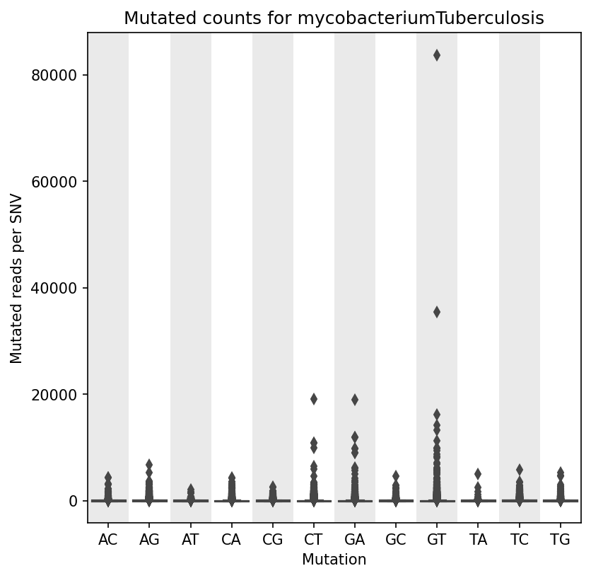
Mutation Count Box Plot
Each sample has its own mutation count box plot, as well as each reference pathogen genome has its own global mutation count box plot. For each possible mutation, it plots the box plot regardless of the position. It is possible to have many outliers, hence the graph can look like a dot plot with a small box in the bottom side. These graphs were stored at 6-visualization/REFERENCE_NAME/graphs/common.mutationCountBoxPlot.png for each reference genome graph, or 6-visualization/REFERENCE_NAME/SAMPLE_NAME/graphs/common.mutationCountBoxPlot.png for each sample.
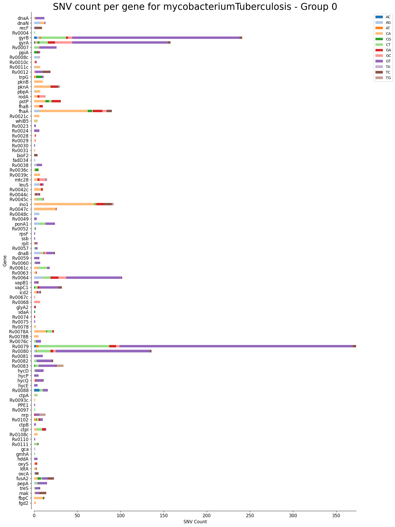
Mutation Count Stacked Bar Plot Per Gene
Each sample has its own mutation count stacked bar plot per gene, as well as each reference pathogen genome has its own global mutation count stacked bar plot per gene. For each gene, it plots a stacked bar, split by each possible mutation, where the length of each bar section is given by the number of reads that mutation has in that gene. It is possible that there are multiple graphs for each sample or reference pathogen. This is because it plots at most 100 genes per file, each file representing a group number. The genes are displayed ordered as they appear in the genome. These graphs were stored at 6-visualization/REFERENCE_NAME/graphs/geneBarPlot for each reference genome graph, or 6-visualization/REFERENCE_NAME/SAMPLE_NAME/graphs/geneBarPlot for each sample. There is also a file named _groups.txt where it says the group number of each gene.
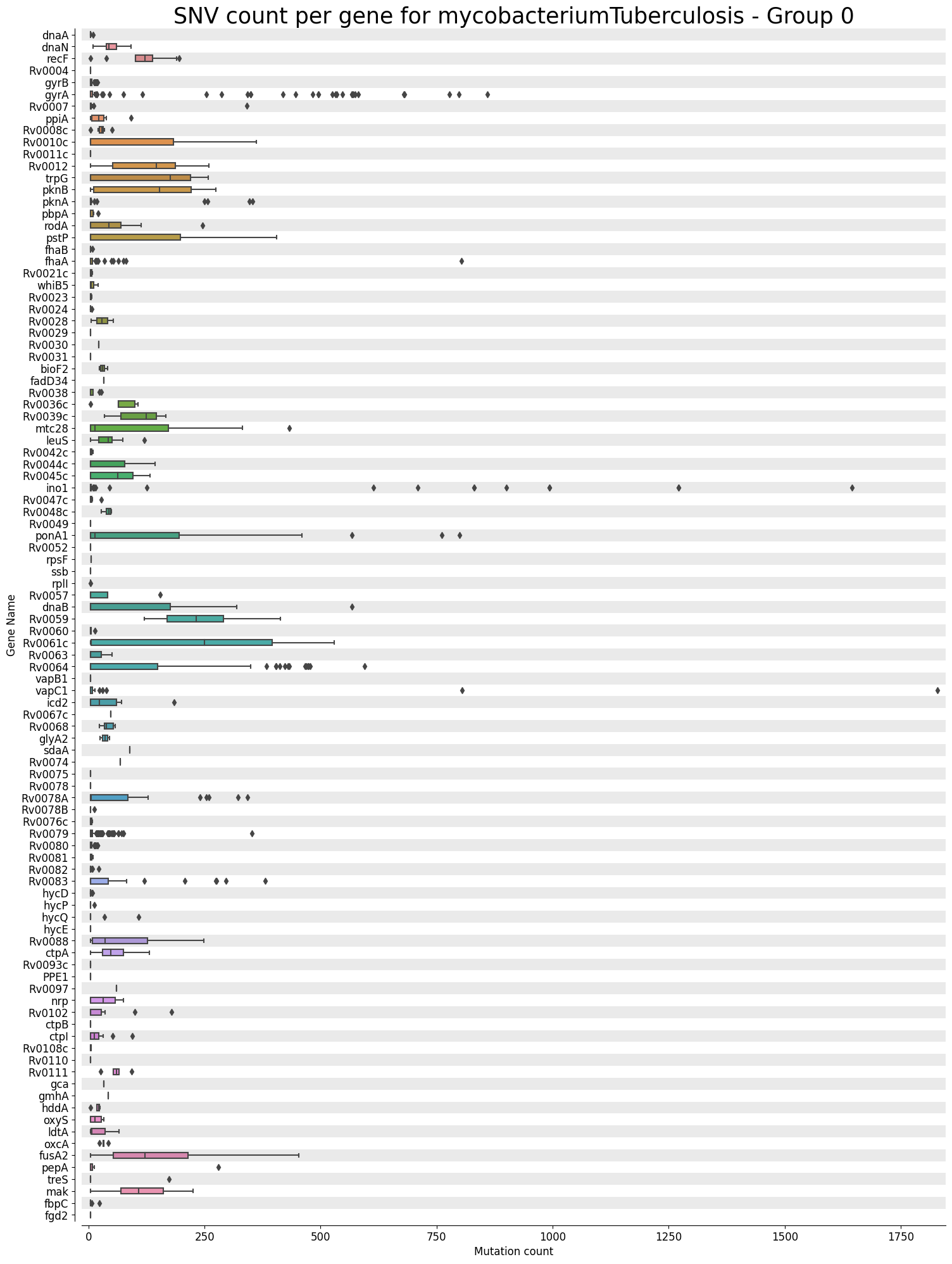
Mutation Count Box Plot Per Gene
Each sample has its own mutation count box plot per gene, as well as each reference pathogen genome has its own global mutation count box plot per gene. For each gene, it plots a box plot based on the number of mutated reads in that gene across all the different positions. Some box plots might have many outliers, so they can look like dot plots with a small box in the left side. It is possible that there are multiple graphs for each sample or reference pathogen. This is because it plots at most 100 genes per file, each file representing a group number. The genes are displayed ordered as they appear in the genome. These graphs were stored at 6-visualization/REFERENCE_NAME/graphs/geneBoxPlot for each reference genome graph, or 6-visualization/REFERENCE_NAME/SAMPLE_NAME/graphs/geneBoxPlot for each sample. There is also a file named _groups.txt where it says the group number of each gene.
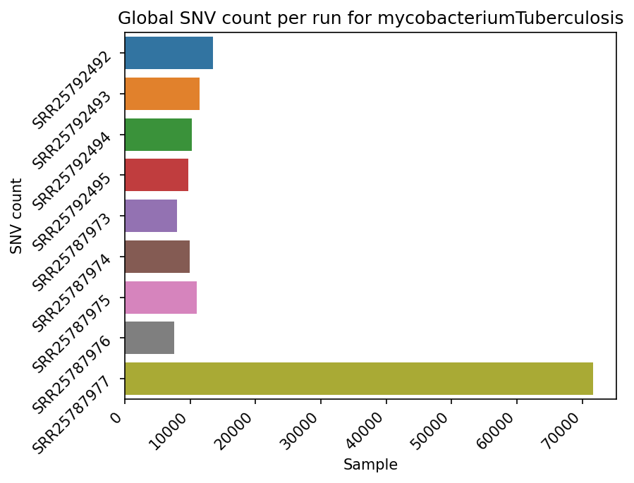
Mutation Count Per Sample Bar Plot
Each reference pathogen genome has its own global mutation count per sample bar plot. For each possible mutation, it counts how many times the mutation happened among all reads in each sample, regardless of the position, and plots it as a bar. Each sample has its own bar. These graphs were stored at 6-visualization/REFERENCE_NAME/graphs/common.mutationsPerRunCountBarPlot.png for each reference genome graph.
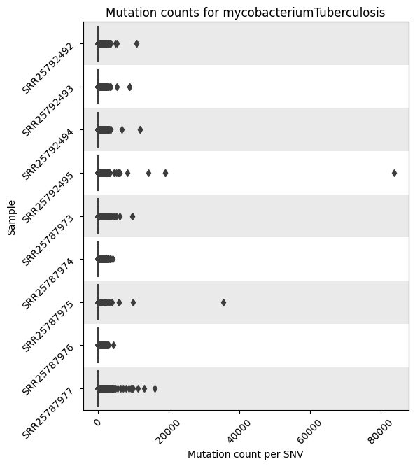
Mutation Count Per Sample Box Plot
Each reference pathogen genome has its own global mutation count per sample bar plot. For each sample, it plots a box plot based on the number of mutated reads in that sample across all the different positions. Some box plots might have many outliers, so they can look like dot plots with a small box in the left side. These graphs were stored at 6-visualization/REFERENCE_NAME/graphs/common.mutationsPerRunCountBoxPlot.png for each reference genome graph.
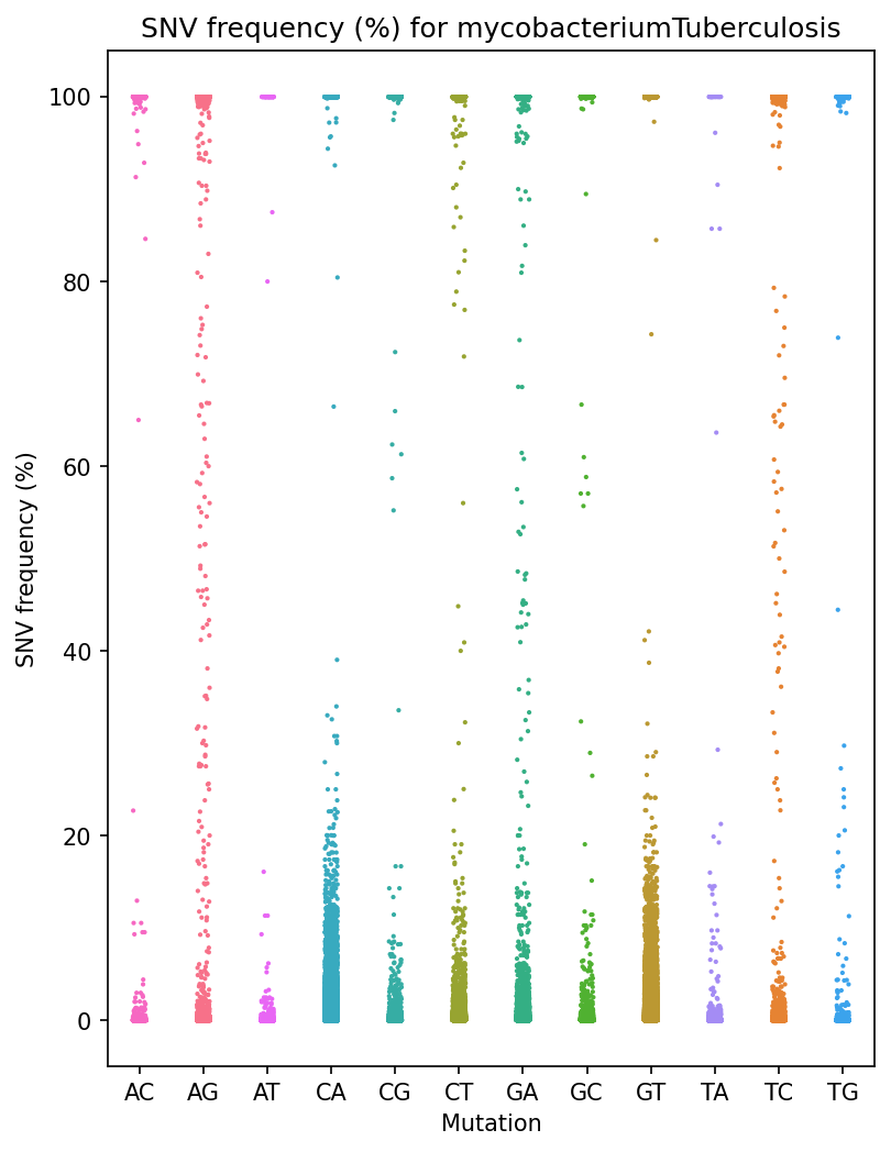
Frequency Per Mutation Strip Plot
Each reference pathogen genome has its own frequency per mnutation strip plot. It plots a strip plot, where each dot is the frequency of an SNV, and it appears in the strip of their respective mutation. These graphs were stored at 6-visualization/REFERENCE_NAME/graphs/common.frequencyPerMutation.png for each reference genome graph.
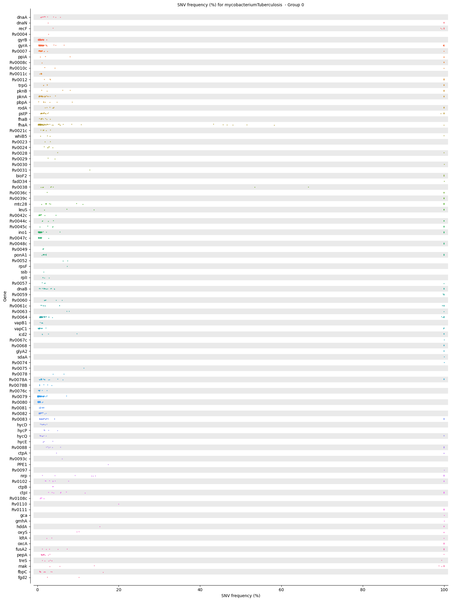
Frequency Per Gene Strip Plot
Each reference pathogen genome has its own frequency per gene strip plot. It plots a strip plot, where each dot is the frequency of an SNV, and it appears in the strip of their respective gene. It is possible that there are multiple graphs for each sample or reference pathogen. This is because it plots at most 100 genes per file, each file representing a group number. The genes are displayed ordered as they appear in the genome. These graphs were stored at 6-visualization/REFERENCE_NAME/graphs/common.frequencyPerMutation.png for each reference genome graph. There is also a file named _groups.txt where it says the group number of each gene.
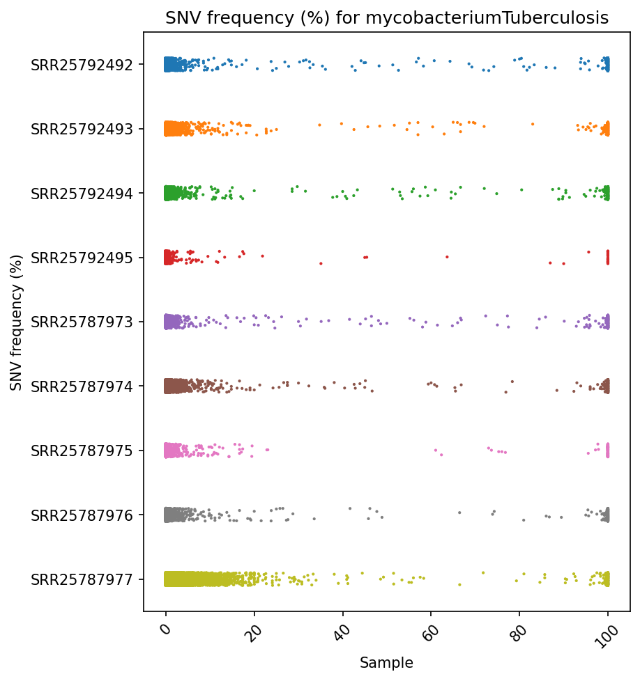
Frequency Per Sample Strip Plot
Each reference pathogen genome has its own frequency per sample strip plot. It plots a strip plot, where each dot is the frequency of an SNV, and it appears in the strip of their respective sample. These graphs were stored at 6-visualization/REFERENCE_NAME/graphs/common.frequencyPerRun.png for each reference genome graph.
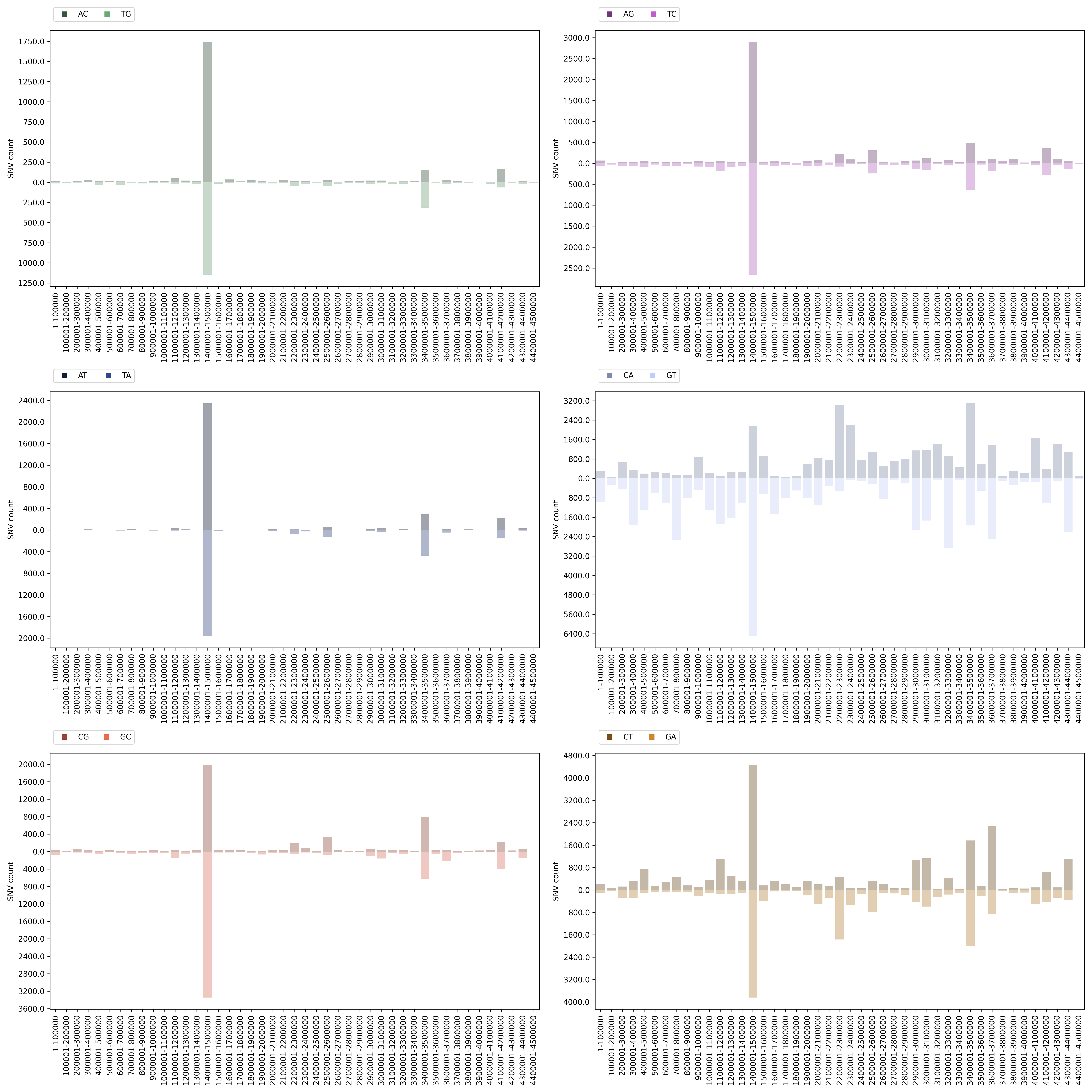
Distribution Histograms Plot
Each reference pathogen genome has its own distribution histograms plots. It plots six graphs in one file per chromosome/segment, where each graph represents a mutation (top half) and its reverse complement (bottom half). Each graph has a histogram displaying the number of SNVs of that mutation found each 100 nucleotides with respect to the reference genome. These graphs were stored at 6-visualization/REFERENCE_NAME/graphs/CHROMOSOME_histogram.png for each chromosome/segment in each reference genome.
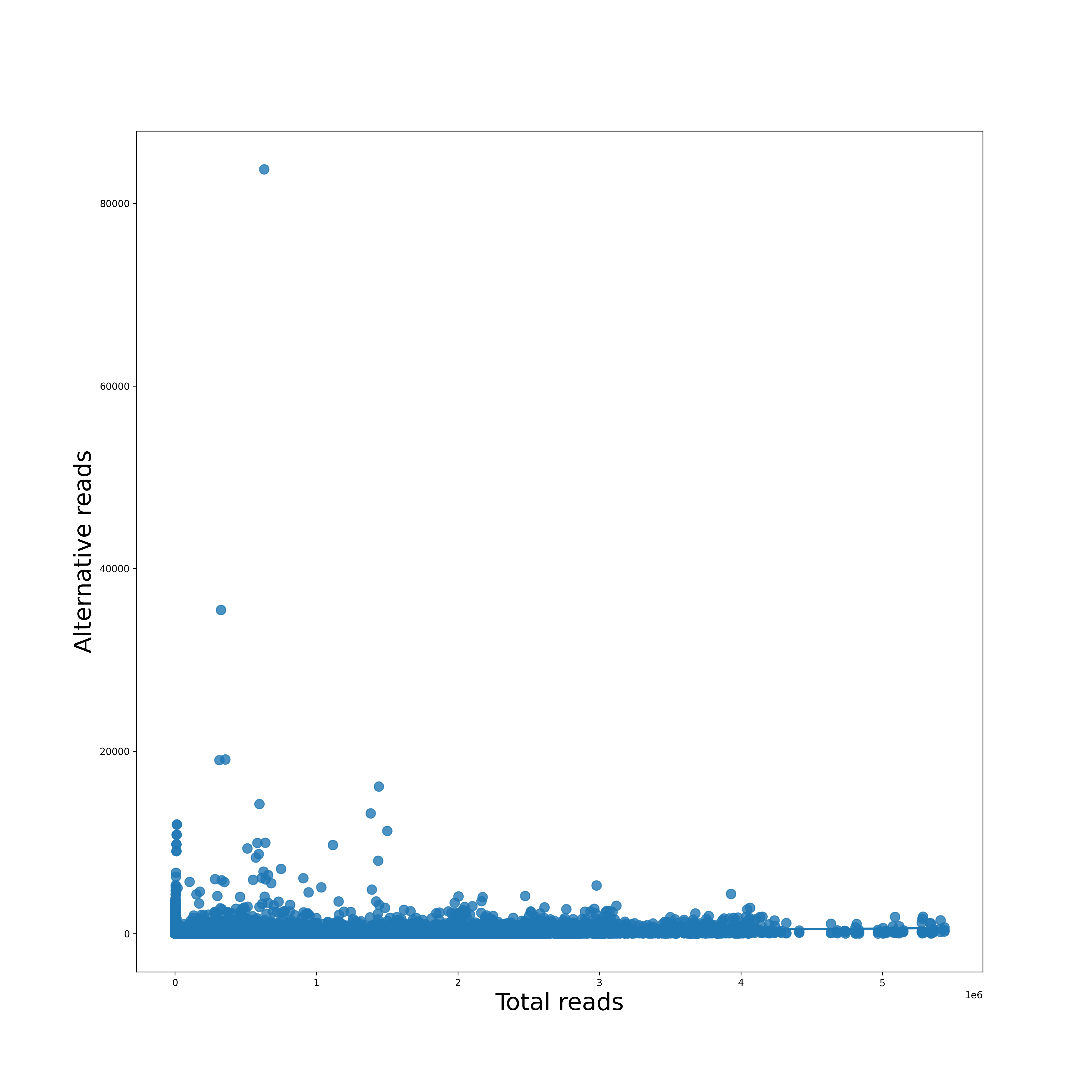
Regression Plot
Each reference pathogen genome has its own regression plots. It displays a dot plot of mutated (or alternate) reads vs the total reads per position. If it finds a suitable linear function, then it is also plotted. These graphs were stored at 6-visualization/REFERENCE_NAME/graphs/CHROMOSOME.regression.png for each chromosome/segment in each reference genome.
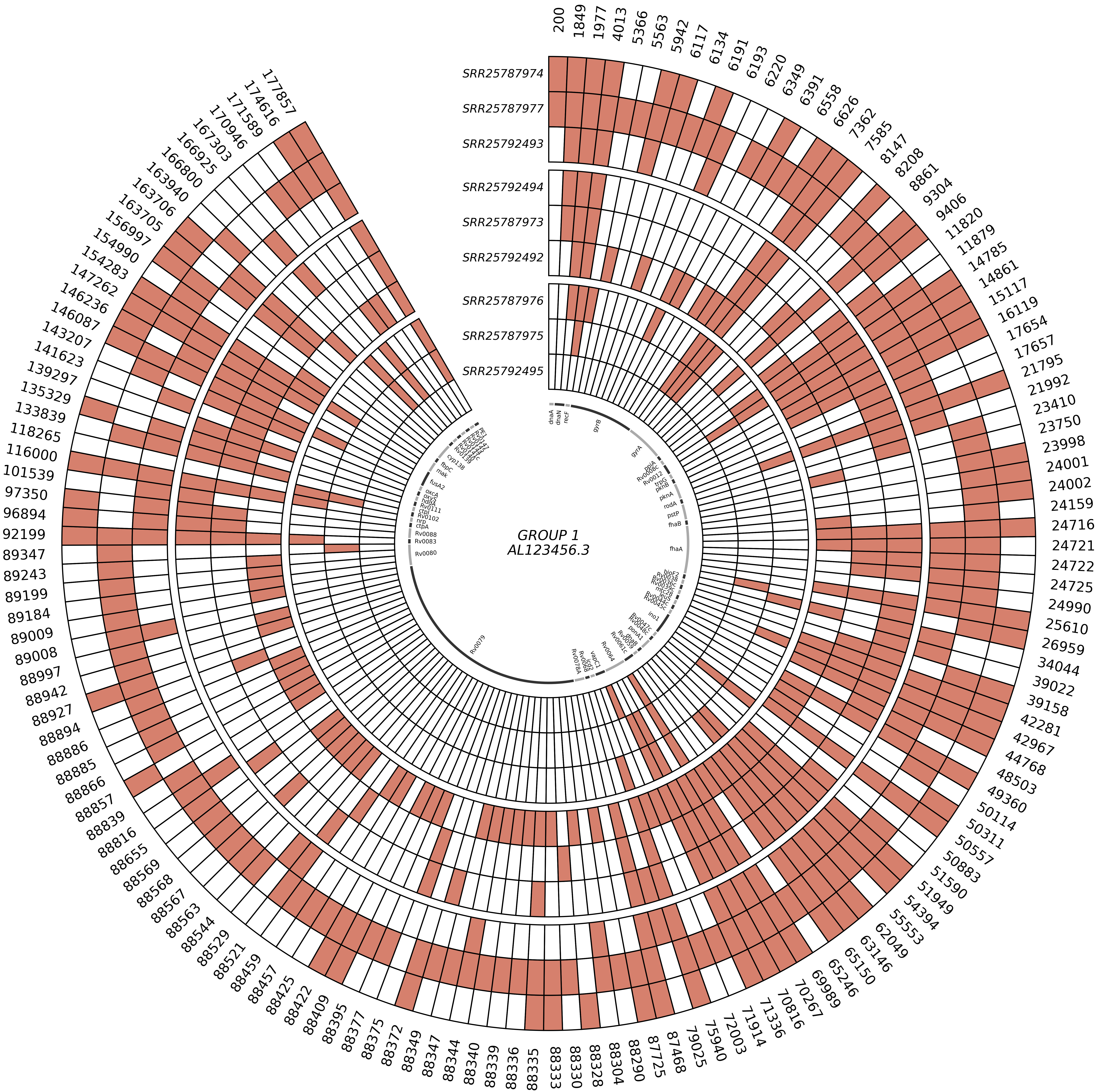
Presence Per Run Position Plot
Each reference pathogen genome has its own presence per run position plots as a circos graph and a heatmap.
The circos graph is a circular graph that displays a different position each arc, up to 150 positions, while each concentric strip at each radius level displays a different run, creating cells. The circos graph supports up to 20 samples. If a cell is colored, then it means that the corresponding position was mutated in that sample. If the graph contains multiple genes, the genes range will be displayed in the innermost circle strip. Because there is a limit on the positions that each circos graph can display, it is possible that there are multiple graphs for each sample or reference pathogen. Genes that have less than 150 mutated positions will be grouped with other genes that also have less than that number of mutated positions. If a gene has more than 150 mutated positions, it will be split in different files. These graphs were stored at 6-visualization/REFERENCE_NAME/graphs/circos/CHROMOSOME_GROUP.png for each group in each chromosome/segment per reference genome, or 6-visualization/REFERENCE_NAME/graphs/circos/GENE_GROUP.png for each group in each gene per reference genome.
The heatmap is a tabular graph where each column represents a sample, and each row represents a position in the reference chromosome/segment. Each heatmap can have up to 300 positions. If a cell is colored, then it means that the corresponding position was mutated in that sample. If the graph contains multiple genes, the genes range will be displayed to the right of the heatmap. Because there is a limit on the positions that each heatmap can display, it is possible that there are multiple graphs for each reference pathogen. Genes that have less than 300 mutated positions will be grouped with other genes that also have less than that number of mutated positions. If a gene has more than 300 mutated positions, it will be split in different files. These graphs were stored at 6-visualization/REFERENCE_NAME/graphs/heatmap/CHROMOSOME_GROUP.png for each group in each chromosome/segment per reference genome, or 6-visualization/REFERENCE_NAME/graphs/heatmap/GENE_GROUP.png for each group in each gene per reference genome.

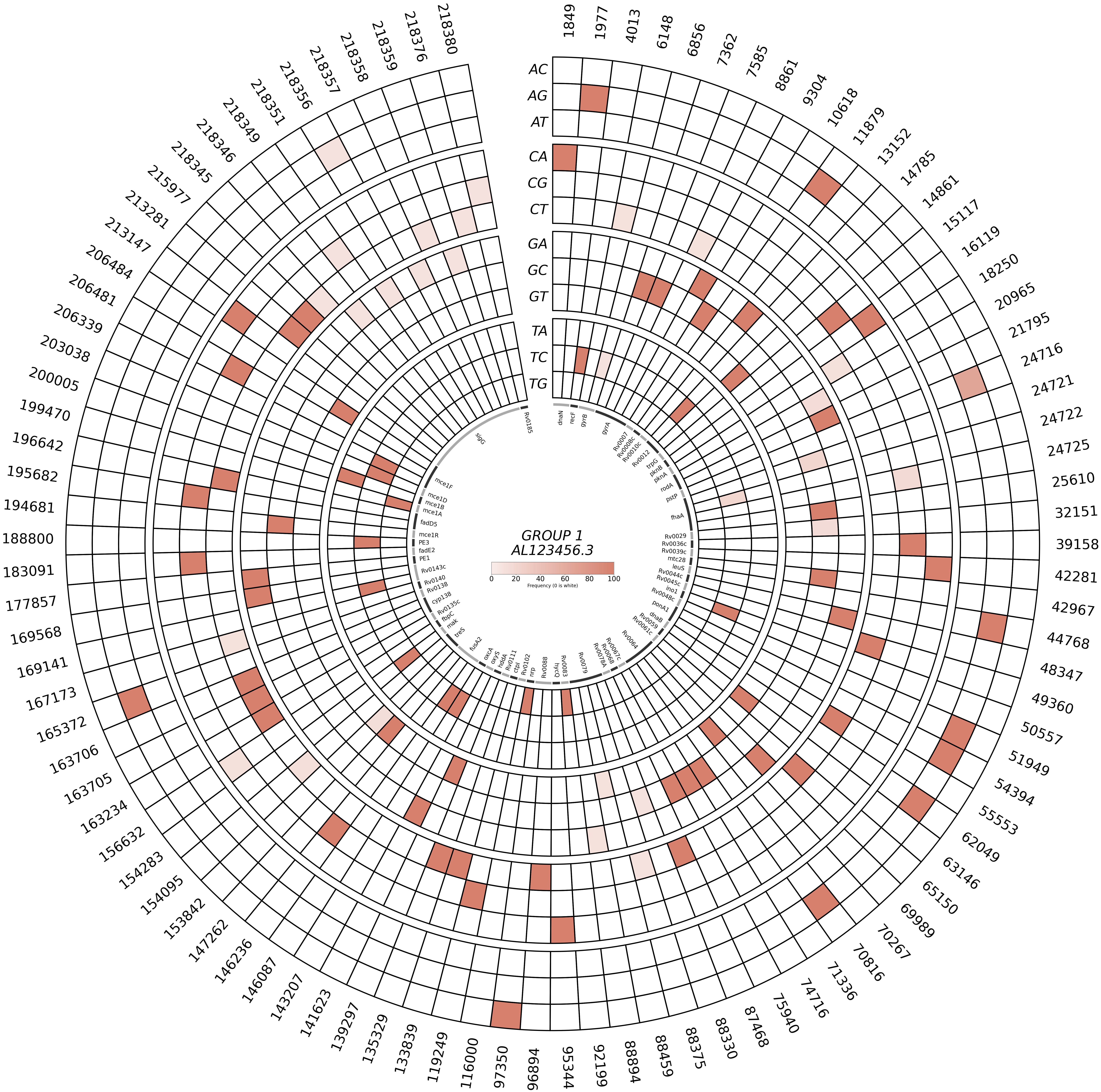
Frequency Per Mutation Position Plot
Each sample has its own frequency per mutation position plots as a circos graph and a heatmap.
The circos graph is a circular graph that displays a different position each arc, up to 150 positions, while each concentric strip at each radius level displays a different mutation, creating cells. If a cell is colored, then it means that the corresponding position had that type of mutation, while the intensity of the color represents the frequency of that position-mutation. If the graph contains multiple genes, the genes range will be displayed in the innermost circle strip. Because there is a limit on the positions that each circos graph can display, it is possible that there are multiple graphs for each sample. Genes that have less than 150 mutated positions will be grouped with other genes that also have less than that number of mutated positions. If a gene has more than 150 mutated positions, it will be split in different files. These graphs were stored at 6-visualization/REFERENCE_NAME/SAMPLE_NAME/circos/CHROMOSOME_GROUP.png for each group in each chromosome/segment per sample, or 6-visualization/REFERENCE_NAME/SAMPLE_NAME/graphs/circos/GENE_GROUP.png for each group in each gene per sample.
The heatmap is a tabular graph where each column represents a sample, and each row represents a position in the reference chromosome/segment. Each heatmap can have up to 300 positions. If a cell is colored, then it means that the corresponding position had that type of mutation, while the intensity of the color represents the frequency of that position-mutation. If the graph contains multiple genes, the genes range will be displayed to the right of the heatmap. Because there is a limit on the positions that each heatmap can display, it is possible that there are multiple graphs for each sample or reference pathogen. Genes that have less than 300 mutated positions will be grouped with other genes that also have less than that number of mutated positions. If a gene has more than 300 mutated positions, it will be split in different files. These graphs were stored at 6-visualization/REFERENCE_NAME/SAMPLE_NAME/graphs/heatmap/CHROMOSOME_GROUP.png for each group in each chromosome/segment per sample, or 6-visualization/REFERENCE_NAME/SAMPLE_NAME/graphs/heatmap/GENE_GROUP.png for each group in each gene per sample.